Once you have a method of describing the serial/parallel structure of an Intel® Cilk™ Plus program, you can begin to analyze the program's performance and scalability.
Consider a more complex program, represented in the following diagram:
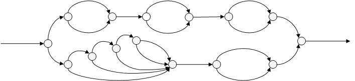
This DAG represents the parallel structure of some Intel® Cilk™ Plus program. To construct a program that has this DAG, it is useful to add labels to the strands to indicate the number of milliseconds it takes to execute each strand:
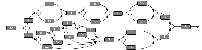
Work
The total amount of processor time required to complete the program is the sum of all the numbers. This value is defined as the work.
In this DAG, the work is 181 milliseconds for the 25 strands shown, and if the program runs on a single processor, the program should run for 181 milliseconds.
Span
The span, sometimes called the critical path length, is the most expensive path that extends from the beginning to the end of the program. In this DAG, the span is 68 milliseconds, as shown in the following diagram:
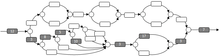
Under ideal circumstances (for instance, when there is no scheduling overhead) and when an unlimited number of processors are available, this program should run for 68 milliseconds.
You can use the work and span to predict how an Intel® Cilk™ Plus program will speed up and scale on multiple processors.
When analyzing an Intel® Cilk™ Plus program, you need to consider the running time of the program on various numbers of processors. The following notations are helpful:
T(P) is the execution time of the program on P processors.
T(1) is the Work
T(∞) is the Span
On 2 processors, the execution time can never be less than T(1) / 2. In general, the Work Law can be stated as:
T(P) >= T(1)/P
Similarly, for P processors, the execution time is never less than the execution time on an infinite number of processors. Therefore, the Span Law can be stated as:
T(P) >= T(∞)
Speed up and Parallelism
If a program runs twice as fast on 2 processors, then the speedup is 2. Therefore, speedup on P processors can be stated as:
T(1)/T(P)
An interesting consequence of the speedup formula is that if T(1) increases faster than T(P), then speedup increases as the work increases. Some algorithms, for example, do extra work in order to take advantage of additional processors. Such algorithms are typically slower than a corresponding serial algorithm on one or two processors, but begin to show speedup on three or more processors. This situation is not common, but is worth noting.
The maximum possible speedup would occur using an infinite number of processors. Parallelism is defined as the hypothetical speedup on an infinite number of processors. Therefore, parallelism can be defined as:
T(1)/T(∞)
Parallelism puts an upper bound on the speedup you can expect. If the code you are parallelizing has a parallelism of 2.7, for example, then you will achieve reasonable speedup on 2 or three processors, but no additional speedup on four or more processors. Thus, algorithms that are tuned to a small number of cores do not scale to larger machines. In general, if parallelism is less than 5-10 times the number of available processors, then you should expect less than linear speedup because the scheduler will not always be able to keep all of the processors busy.